How a Diffusion Transformer Generates Shapes from Text
An interactive guide to Diffusion Transformers and Flow Matching, using a simple model that turns random dots into shapes.
Image models like Stable Diffusion 3 and FLUX rely on a Diffusion Transformer (DiT) paired with Flow Matching. This article uses a simple DiT model to illustrate the core mechanics behind these systems.
Given a prompt like circle on triangle, generation begins with 24 random points. The model moves them step by step. In the end, the points form the outlines of the scene described in the prompt.
Demo
Prompts can name a single shape, like circle, or combine two shapes with a spatial relation, like circle on square.
Every prompt is composed of up to 4 tokens, drawn from a 12-word vocabulary:
- Shapes:
dot, circle, triangle, square - Relations:
on, above, under, below, left, right, of - Padding:
PAD(fills unused slots)
Architecture
The model works in three stages: embedding, attention, and projection.
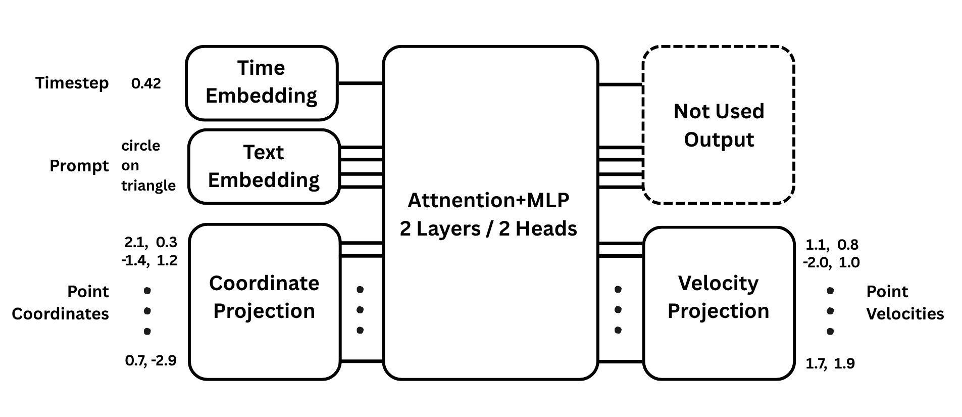
Diffusion Transformer (DiT) architecture
The model receives three types of inputs. Each is mapped to a 64-dimensional vector:
- 1 Timestep: Tells the model where it is on the path from noise to shape. Encoded with sinusoidal encoding.
- 4 Text tokens: Contain the prompt words. Encoded with learned word embeddings and positional encodings.
- 24 Coordinate points: Represent the (x, y) positions at the current timestep. Projected using a linear layer.
The model merges these vectors into a single 29-token sequence and passes them through 2 transformer layers. Each layer runs self-attention with 2 heads, followed by an MLP.
The output layer turns each of the 24 point tokens into a velocity, the direction from shape to noise. The points are moved slightly in the opposite direction. Repeating this process forms the shape.
Timestep Embedding
To predict the direction, the model must know where the points are on their path from noise to shape. The timestep indicates this progress as it decreases from 1 to 0. The value is encoded with sine and cosine waves, called sinusoidal encoding. Most waves barely move over such a small range, so is scaled by 100 first. The result is a 64-dimensional vector:
Here, D = 64 is the dimension, k runs from 0 to 31 for each sine-cosine pair, and base b = 500 sets the frequency range.
Plotted in 3D, the components form a landscape of waves across time. The sliders show how the base and the dimension reshape it:
Sinusoidal encoding. Each ridge shows how an individual component changes over 100 timesteps.
Close timesteps should get close vectors. In vector space, similarity is measured with the dot product. Pairing sine with cosine makes this similarity depend only on the time difference. Consider two 2D encodings and , in this case with . Their dot product simplifies via the angle difference identity:
Both vectors have length 1, so the dot product is their cosine similarity. While a single wave repeats every few steps, combining 32 frequencies makes the similarity fall as the timesteps move apart.
The encoding works like a clock with 32 hands. Each sine and cosine pair sets the position of one hand. Just as humans use hours, minutes, and seconds instead of counting only seconds, the network processes time more easily when split across multiple frequencies.
Shorter hands represent high frequencies and spin quickly, while longer hands represent low frequencies and turn slowly.
Text Embedding
The model uses the prompt to know which shapes to draw and where to place them. Each prompt has a fixed length of 4 tokens from a 12-word vocabulary. A learned embedding table maps each token to a 64-dimensional vector. Unused slots are filled with PAD.
A positional encoding is added to each vector so the model can tell the difference between triangle on circle and circle on triangle.
Instead of learned positional embeddings (as in How a Transformer Plays Tic-Tac-Toe), the model follows the original Attention Is All You Need paper and uses sinusoidal encoding (with base b = 10).
Coordinate Projection
The third input is the coordinates of 24 points at timestep . A learned linear layer with weights and biases projects each coordinate pair into a 64-dimensional vector:
Note: Matrix multiplications visualized as a row–column diagram. Rows are separated to show each token is processed independently.
Attention Patterns
Attention is where tokens exchange information. The mechanics of queries (Q), keys (K), and values (V) are covered in How a Transformer Plays Tic-Tac-Toe.
The model has 2 layers with 2 heads each, a width of D = 64, and a context length of 29 tokens. Every point can attend to all other points, the prompt words, and the timestep. The only mask hides the empty PAD slots in the prompt.
In the last steps of generation, the second layer shows a distinct role for each head:
- Head 1 assigns points to shapes. Points attending to "triangle" form the triangle on the canvas, while points attending to "circle" form the circle.
- Head 2 tracks neighboring points. Each row shows three or four activations: the point itself on the diagonal, plus its left and right neighbors along the outline.
Click inside the green box to highlight where the corresponding points are located.
Velocity Projection
The timestep and prompt tokens have conditioned the points in attention and are no longer needed. The model keeps only the 24 point vectors.
A final linear layer with learned weights and biases projects each point vector to a 2D velocity: the direction from the shape toward noise.
Each point then moves the opposite way, from noise toward the shape, and the timestep decreases. The model runs again on the updated points and timestep. The loop repeats until .
Flow Matching
Flow Matching connects clean shapes and random noise with straight lines. The forward process moves from shape to noise and is used in training. The reverse process moves from noise to shape and is used in generation. Both processes are described by the same formula:
Here, is the clean shape, is random noise, and represents the points at timestep .
Forward Process
In the forward process, time runs from 0 to 1. As increases, the shape signal scales by while the noise contribution scales by .
Solid black dots represent the current points, while faint gray circles show their destination noise positions.
The points move in straight lines. The model learns to predict the direction of these lines, called the velocity:
Arrows represent the velocity vectors, pointing from each shape point to its corresponding noise position.
Reverse Process
The main formula can be rewritten in terms of the velocity :
This formula can be rewritten in recursive form to calculate the position of the points at the previous step, :
Generation starts at , where is pure noise. The model predicts the velocity , and the recursive formula calculates the next positions of the points, . Repeating this step gradually forms the shape.
Move the vertical slider to inspect different trajectories.
Time Shifting
Generation can use any number of steps: more steps trace the path more accurately, while fewer steps run faster.
Early models spaced these steps evenly from 1 to 0. Later systems introduced time shifting to concentrate steps where the model needs the most precision.
A shift factor maps the evenly spaced times to new times :
At , nothing changes. Setting puts more steps near noise, while puts more steps near the shape.
Training
The training set contains 100K samples generated by a script. Each sample pairs a text prompt with the coordinates of 24 points. Half the samples show a single centered shape. The other half pair two shapes using a spatial relation. All prompts that describe a circle on a triangle were excluded on purpose to test generalization.
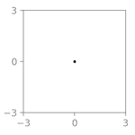
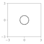
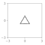
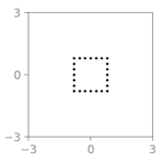
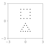
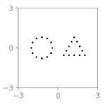
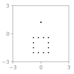
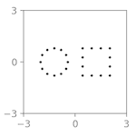
Training samples with single shapes and shape pairs (circle-on-triangle scenes excluded).
Each training step starts with three components: a clean sample from the dataset, a random timestep between 0 and 1, and random noise .
The forward formula mixes them into the noisy points . The velocity formula gives the target from the same and .
The model receives , the timestep, and the prompt, and predicts the velocity. The prediction is compared against the target using mean squared error (MSE) loss.
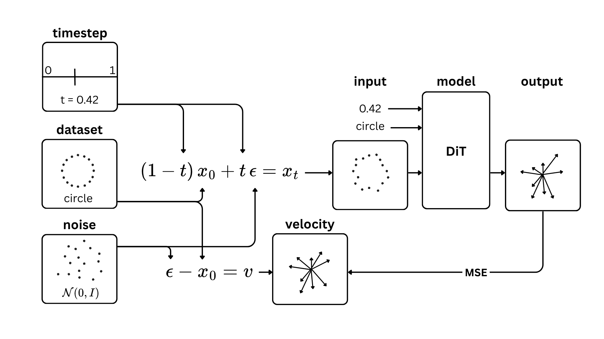
is the standard notation for Gaussian noise with mean 0 and variance 1.
The full training code is available in the Jupyter notebook.
Generalization
Instead of memorizing fixed scenes, the model learns shapes and spatial relations as independent concepts.
For example, the prompt circle on triangle generates the scene correctly, even though the model never saw it during training.
The model can also blend shapes. For instance, the prompt square triangle produces a trapezoid.
Here are some examples not present in the training set:
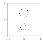
circle on triangle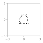
triangle square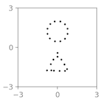
triangle below circle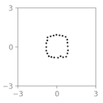
square circleOut-of-distribution prompts can be tested in the demo above.
This ability to combine separate concepts is called compositional generalization. It allows real image models to generate scenes never seen during training, like "a pelican riding a bicycle" or "an astronaut riding a horse".
Conclusion
The model in this article uses the same core ideas as text-to-image systems like Stable Diffusion 3 and FLUX: text and time conditioning, transformer attention between image and prompt tokens, and Flow Matching.
Production systems scale these ideas in four main ways:
| 2-layer DiT | Production systems | |
|---|---|---|
| Text | 12-word vocabulary | Pretrained encoders such as T5 and CLIP turn full text prompts into vectors. They already know language, so the model understands long and detailed prompts. |
| Images | 24 points representing shapes | An autoencoder compresses RGB pixel values into a compact latent representation. The model works on the latent, not on raw pixels. This allows high-resolution images. |
| Architecture | 2 layers, D = 64, context = 29 | Over 20 layers, D above 1500, and a context of over 4000 tokens. The added capacity captures more complex image-text relationships. |
| Data | 100K synthetic samples | Trained on billions of web images, with descriptions parsed from alt attributes or generated by vision-language models such as CogVLM. |
Generation works the same way for real images. The model starts with noise and gradually transforms it into an image that matches the text prompt.
A Visual Introduction to Rectified Flows article goes deeper into the math of Flow Matching. It shows why sampled trajectories curve and how Rectified Flow straightens them. The video by Welch Labs on the 3Blue1Brown channel gives a bigger picture of diffusion models. It covers DDPM and DDIM sampling from early diffusion models, CLIP text-image embeddings, conditioning, and other topics.